Photometric RM#

mica2 provides a pmap mode to do photometric reverberation mapping analysis, which aims at singling out the reverberation of broad emission lines in photometric light curves that are generally dominated by the continuum variations. The adopted transfer function consists of two components, namely, for Gaussians,

\[\Psi(\tau) = \frac{f_1}{\sqrt{2\pi}\omega_1} \exp\left[-\frac{(\tau-\tau_1)^2}{2\omega_1^2}\right] +\frac{f_1 R}{\sqrt{2\pi}\omega_2} \exp\left[-\frac{(\tau-\tau_2)^2}{2\omega_2^2}\right],\]

or for tophats,

\[\Psi(\tau) = \frac{f_1}{2\omega_1} H(\tau, \tau_2, \omega_2) +\frac{f_1 R}{2\omega_2} H(\tau, \tau_2, \omega_2),\]

where \(f_1, \tau_1, \omega_1\) are for continuum reverberation and \(R, \tau_2, \omega_2\) are reverberation of the broad emission line. Here \(R\) represents the fraction of responses relative the continuum component.

mica2 assumes that the driving photometric light curve does not contains line emissions and represents pure continuum variability.

In the exectuable binary version, the typical parameter file looks like:

#
# lines starting with "#" are regarded as comments and are neglected
# if want to turn on the line, remove the beginning "#"

#==============================================================

FileDir                       ./
DataFile                      data/sim_data.txt

TypeModel                     1            # 0: general model
                                           # 1: pmap, photometric RM

TypeTF                        0            # 0: Gaussian
                                           # 1: Top-hat

MaxNumberSaves                2000         # number of steps
FlagUniformVarParams          0            # if each data set has the same variability parameters
FlagUniformTranFuns           0            # if each data set has the same tf parameters
FlagLongtermTrend             0            # if long-term trending

FlagLagPositivity             0            # if enable tf at positive lags
NumCompLow                    2
NumCompUpp                    2

FlagConSysErr                 0
FlagLineSysErr                0

StrLagPrior                   [0.000000:10.000000:10.000000:50.000000]  # prior range of lags of each components
StrRatioPrior                 [1.0e-3:0.5]                              # response ratio prior of line component

For python version, mica provide a module pmap callable as follows.

from mpi4py import MPI
import numpy as np
import pymica
import matplotlib.pyplot as plt

# initiate MPI
comm = MPI.COMM_WORLD
rank = comm.Get_rank()

# load data
band1 = np.loadtxt("g.txt")
band2= np.loadtxt("r.txt")

# make a data dict
data_input = {"set1":[band1, band2]}
# if multiple datasets, e.g.,
#data_input = {"set1":[con1, line1], "set2":[con2, line2]}
# if a dataset has multiple lines, e.g.,
#data_input = {"set1":[con, line1, line2]}

#create a model
#there are two ways
#1) one way from the param file
#model = pymica.gmodel(param_file="param/param_input")

#2) the ohter way is through the setup function

model = pymica.pmap()
model.setup(data=data_input, type_tf='gaussian', max_num_saves=2000, lag_prior=[[-5, 5],[0, 50]], \
            ratio_prior=[[0.05, 0.5]])

# if using tophats, set type_tf='tophat'

#the full arguments are
#model.setup(data=data_input, type_tf='gaussian', max_num_saves=2000, \
#            lag_prior=[[-5, 5],[0, 50]], ratio_prior=[[0.05, 0.5]],\
#            flag_con_sys_err=False, flag_line_sys_err=False, \
#            width_limit=[0.01, 100])

#run mica
model.run()

#posterior run, only re-generate posterior samples, do not run MCMC
#model.post_run()

#do decomposition for the cases of multiple components
#model.decompose()

# plot results
if rank == 0:

  model.plot_results() # plot results
  model.post_process()  # generate plots for the properties of MCMC sampling

Here is an example for pmap analysis. The data is extracted from Fausnaugh et al. 2018, ApJ, 854, 10.

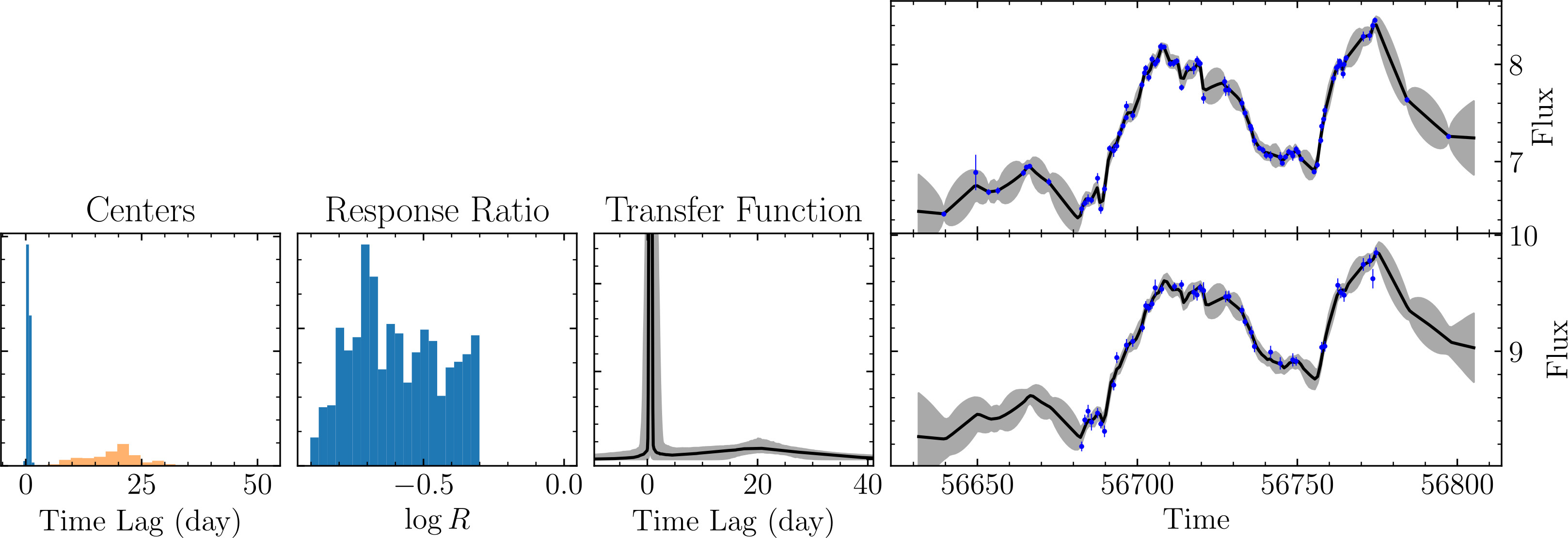
_images/fig_pmap.jpg — An examplary result of MICA2 analysis with pmap mode.#