Tests#
Make sure that your MICA compiling is successful. After that, change to the subdirectory tests.
There are a suite of tests provided
python: a python example
twogauss: the transfer function consists of two Gaussians
twotophat: the transfer function consists of two top-hat
gamma: the transfer function is gamma type
exp: the transfer function is exponential type
pmap: photometric reverberation mapping
vmap: virtual reverberation mapping
mmap: reverberation mapping with a mixture of transfer function types
negative_resp: the transfer function can be negative
restart: resume from a last run
Change to any one folder and run the test to get familar with the useage of MICA.
I. python#
This test provides an example for the useage in Python. Run the Python script as
mpiexe -n 6 python example.py
Here 6 cores are used. If one wants to use other number of cores, change the number accordingly.
This test is indeed same with the twogauss test below.
II. twogauss/twotophat#
These two tests use the executable binary version mica. A shell script is provided to run the code and plot the results.
Run the shell script as
./test_twogauss.sh
or
./test_twotophat.sh
The script will create folders data and param, place appropriate files in the two folders, copy
the executable file mica2 and ploting script plotfig.py, and then run mica2 and plot the results.
Here is the output for the twogauss tests.
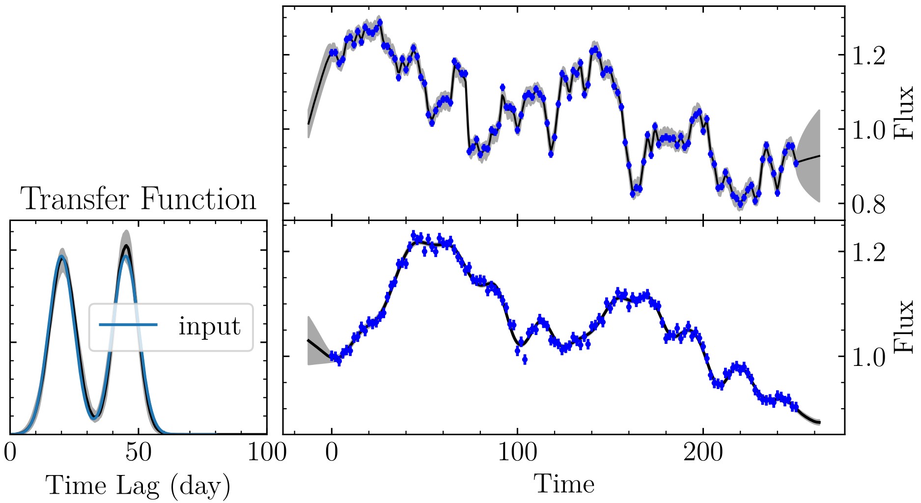
Results using two Gaussians. (Left) transfer functions; (Right) Fits to light curves.#
The obtained evidences are:
# number_of_gaussians     ln(evidence)
1       673.680528
2       814.866840
It is clear that the case of two Gaussians are decisively perferred over the case of one Gaussian. The obtained transfer function is remarkably consistent with the input.
Note
MICA does not take into account a constant normalization factor for the likelihood function, so the obtained Bayesian evidence might be larger than 1. In this case, only the differences in evidence make sense.
III. gamma#
The transfer function is a gamma function (k=2). Run the Python script as
mpiexe -n 6 python example.py
Here 6 cores are used. If one wants to use other number of cores, change the number accordingly.
The output plot looks like

The results for a test with gamma transfer function.#
IV. exp#
The transfer function consists of two exponential functions. Run the Python script as
mpiexe -n 6 python example.py
Here 6 cores are used. If one wants to use other number of cores, change the number accordingly.
The output plot looks like
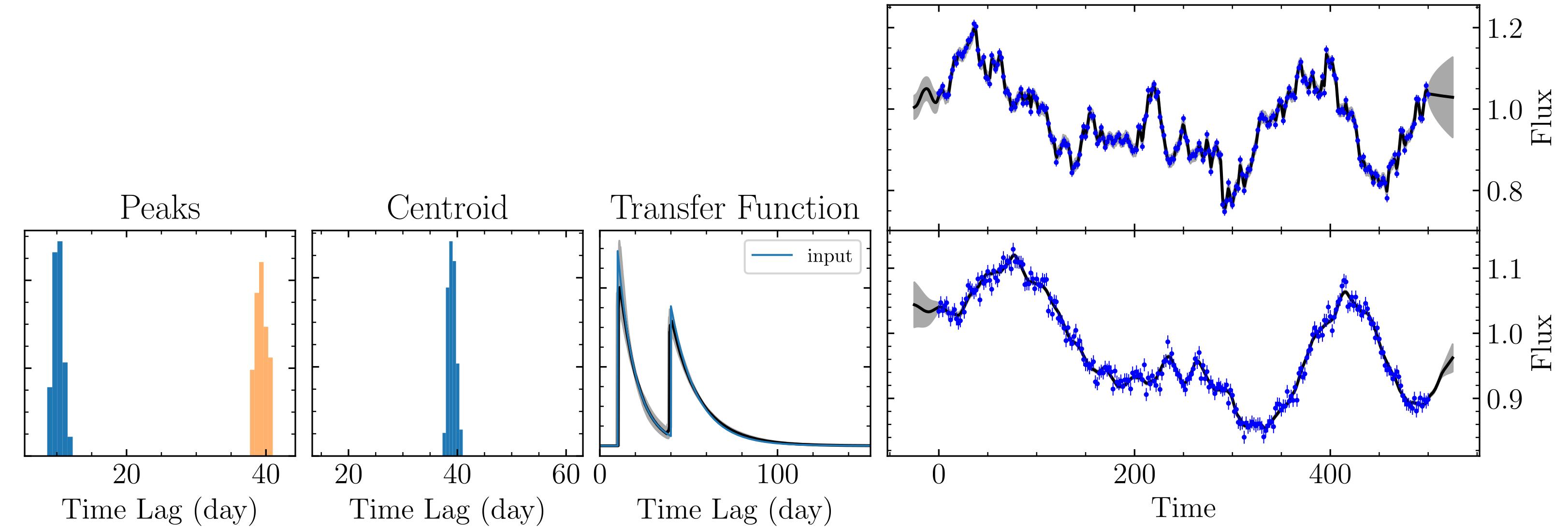
The results for a test with exponential transfer function.#
V. pmap#
Please refer to Photometric RM to see the detail.
VI. vmap#
Please refer to Virtual RM to see the detail.
VII. mmap#
The transfer function consists of two different types of basic functions. MICA2 supports an abitrary number of components. Here two components are used for illustration purpose. Run the Python script as
mpiexe -n 6 python example.py
Here 6 cores are used. If one wants to use other number of cores, change the number accordingly.
The output plot looks like
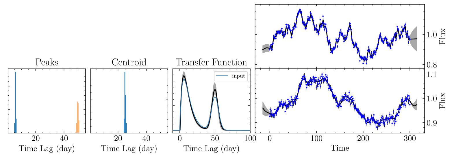
The results for a test with a mixture of Gamma and Gaussian transfer functions.#
VIII. negative_resp#
Please refer to Negative Responses to see the detail.